How to Filter the General Ledger Using Google Sheets
Filtering the general ledger allows you to easily see multiple accounts and sub accounts within Proximity - such as all of your processing fees in a given time period, all of your custom charges, all of the processing fees collected from members, and more. The following article will explain how to do this using Google Sheets.
Download the Ledger as a CSV
Navigate to Reports > Ledger Export.
- Choose the time period.
- Select Download CSV.
Import the Ledger as a Spreadsheet
- Open a blank Google Sheets.
- File > Open > Select the downloaded ledger file.
Expand All Cells to Fit to Data
This will resize all cells to include all information in the cells.
- Select the first column header (A) + shift + the last column header (N in this example.)
- Select Resize Column A-N.
- Check the box next to Fit to Data.
- Select Ok.
Format the Spreadsheet to the Filter View
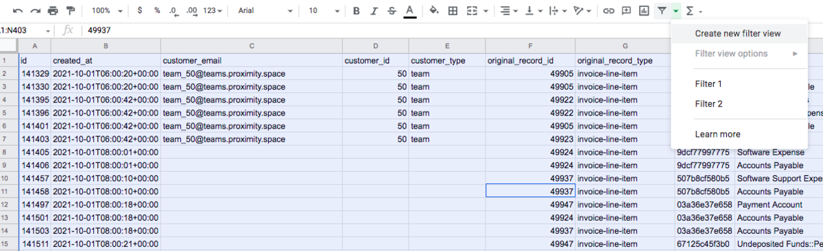
- Select all. (command + a on mac, ctrl + a on pc)
- Select the Filter button (second to last button on the right that looks like a funnel)
- Select Create New Filter View.
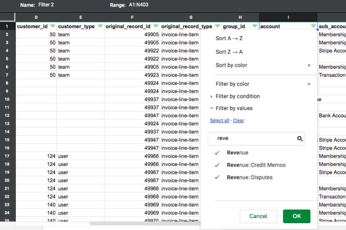
This view allows you to filter out or hide rows by filtering the column. To filter a column, you will select the upside-down pyramid button at the top of a column. You will want to clear the filter, then type in a value to filter the spreadsheet.
For example, if you are wanting to filter the accounts column to show you all revenue, you would select "Clear" then type in "Revenue" and select all accounts including revenue.
Create a Subtotal Cell for Credit/Debit Columns
Adding a cell for the subtotals (rather than the SUM) will allow you to see the subtotals of the credit and debit columns as you filter the spreadsheet. The subtotals will exclude any hidden cells in the spreadsheet. This allows you to easily add up the columns to see the totals debited and credited in to the filtered accounts and sub accounts.
- At the very bottom of the Debits column, select a cell outside of the box that is created by the filter view.
- Type: "=SUBTOTAL(109, M2:M[[the last row for the debit column]]"
- In the example, below, the last row is 403 so the formula for the subtotal of the Debits column is "=SUBTOTAL(109, M2:M403)"
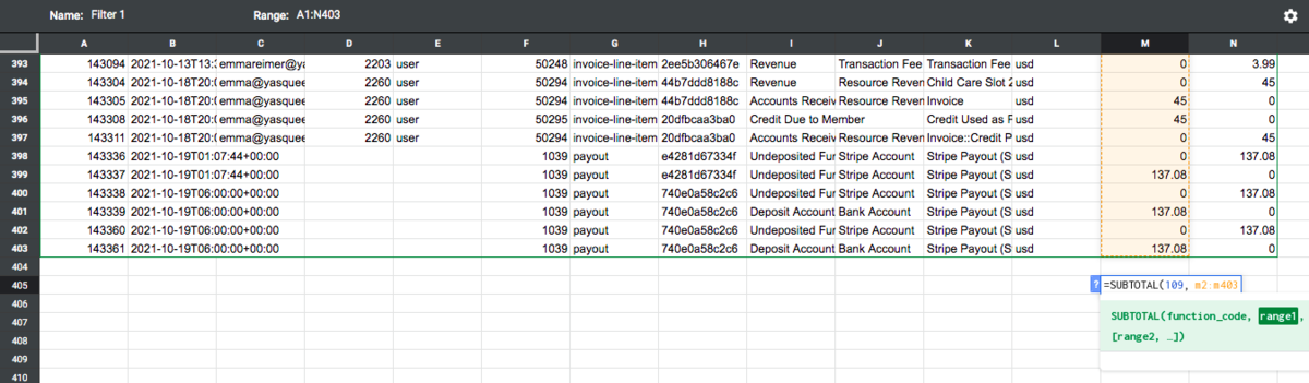
- Type the same formula at the bottom of the Credits column.
- In this example, the formula would be "=SUBTOTAL(109, N2:N403)"
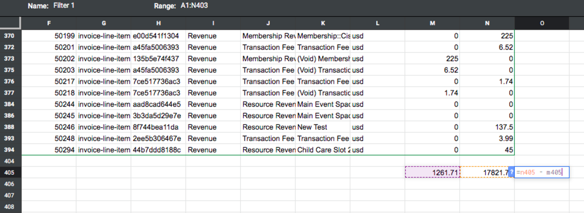
- You can go one step further and create a cell next to your subtotals to subtract your debits from your credits.
- In this example, the formula would be "=n405 - m405" (n405 is the cell with the subtotals for the credits, m405 is the cell with the subtotals for the debits.)
- Now when you filter by all revenue accounts, you will get an exact number of all revenue from that period in this cell.